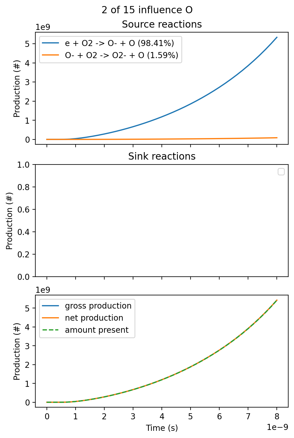
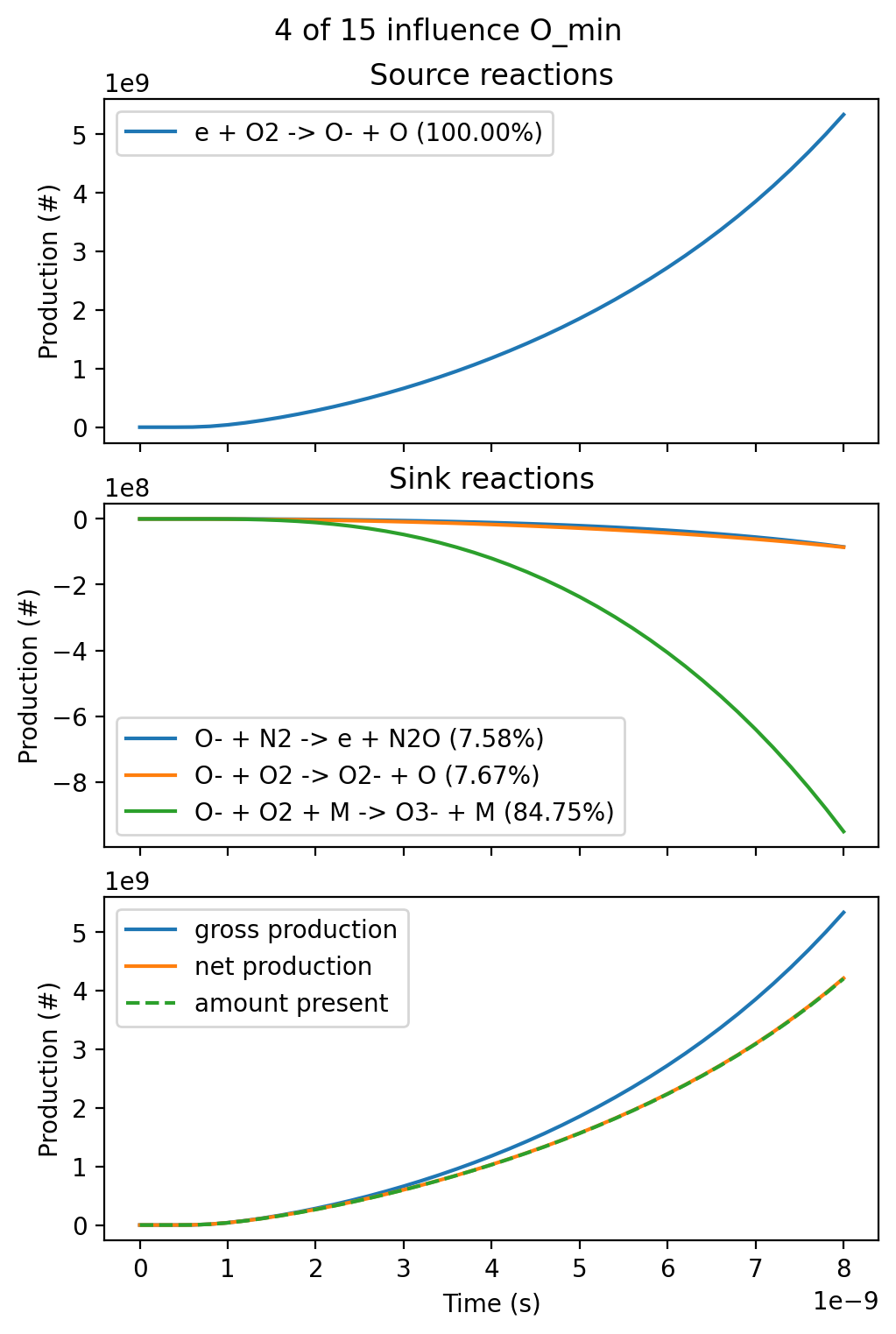
In this example, we will run a 2D axisymmetric simulation and analyze the production of varies species, as well as the energy deposited into the discharge. A config file is provided at tutorials/species_production/air_cyl.cfg. In this example, we focus on the production of atomic oxygen on nanosecond time scales.
Visualizing the production of atomic oxygen
The script chemistry_visualize_rates.py (see python tools) can show the production of a species over time. After running the simulation, the script can be executed as
../../tools/chemistry_visualize_rates.py output/air_cyl_rates.txt -soi O
where ../../tools depends on the current working directory. The graphical output of the script for the production of O and O- is shown below:


These figures show several quantities:
- Which reactions produce the species (source reactions), and their relative contributions
- Which reactions remove the species (sink reactions), and their relative contributions
- The amount of the species (in number of molecules) that is present over time. This is (approximately) equal to the integrated 'net' production of the species over time if the initial density was zero
- The total gross production of the species, not accounting for losses
Determining the energy cost per molecule
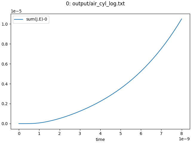
A good approximation of the total energy deposited into the discharge is given by the integral over time and space over the Joule heating term \(\mathbf{J} \cdot \mathbf{E}\). This quantity is saved in the log file (see Saving output and visualization), and can for example be plotted using the plot_log_xy.py script:
../../tools/plot_log_xy.py output/air_cyl_log.txt -x time -y 'sum(J.E)'
which produces the following output

From the graphical output, we can estimate that about 1e10 oxygen atoms were produced (half O, half O-), for a total energy input of about 1e-5 Joule, which means that on the order of 6e3 eV was used per oxygen atom. This is a way higher number than one would normally expect, which is caused by the fact that the used chemistry did not include dissociation reactions of the form
e + O2 -> e + O + O
An important lesson is therefore to always check whether the chemistry contains the appropriate reactions for a particular study!